Sound Level Metrics Distributions#
Learning Objectives
Summarize the distribution of sound levels from a hydrophone through a histogram.
Compute the empirical probability of an event from the histogram.
Here we will explore the distribution of ocean sound levels from a hydrophone recording. We will access data from the Sanctuary Soundscape Monitoring Project which is publicly available through the NOAA NCEI Passive Acoustics Archive. We will use a dataset of computed broadband sound levels at 1 hour intervals.
import pandas as pd
import matplotlib.pyplot as plt
sound_levels = pd.read_csv("https://storage.googleapis.com/noaa-passive-bioacoustic/sanctsound/products/sound_level_metrics/oc03/sanctsound_oc03_02_bb_1h/data/SanctSound_OC03_02_BB_1h.csv")
# summary statistics of the dataset
sound_levels.describe()
| BB_20-24000 | |
|---|---|
| count | 3003.000000 |
| mean | 103.586356 |
| std | 7.508545 |
| min | 85.349354 |
| 25% | 98.694873 |
| 50% | 103.723633 |
| 75% | 108.123486 |
| max | 134.773183 |
Histogram#
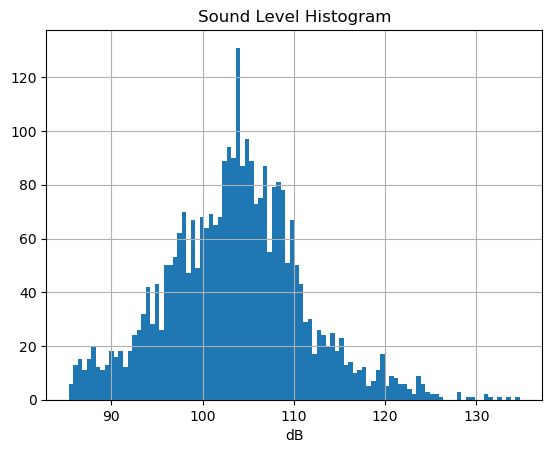
Looking at the histogram of the data provides a good first glance of the distribution of the observations.
h = sound_levels.hist(bins=100)
plt.xlabel("dB")
_ = plt.title("Sound Level Histogram")
Note
We observe that the range of the values is approximately (85 dB, 135 dB). Since those are averaged over 1 hour windows, the actual observed values can fall outside this range.
We also observe that the distribution looks skewed which is typical for sound level distributions. The upper tail is long, which corresponds to rare observations of loud sounds.
Computing Empirical Probability#
The empirical probability of an event is the relative frequency of the event, or the proportion of trials for which the event occurred.
Example: compute the probability of the event sound levels > 120 dB.
# let's calculate the proportion of the values

# note the BB_20-24000 column name has spaces around it!

sum(sound_levels[" BB_20-24000 "]>120)/len(sound_levels)
0.024642024642024644
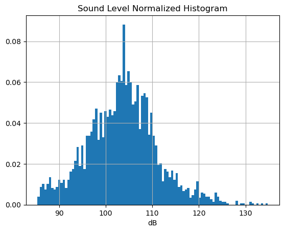
The histogram splits the range of the outcomes into small intervals (bins) and computes the frequency of the observed outcomes in each bin. Thus, if we compute the normalized histogram (each frequency is divided by the total number of observations), we can use it to estimate the empirical probability that the sound level falls within a particular interval (by summing the frequency for the bins falling in this interval).
# Set density=True to plot normalized histogram
h = sound_levels[' BB_20-24000 '].hist(bins=100, density=True)
plt.title("Sound Level Normalized Histogram")
_ = plt.xlabel("dB")
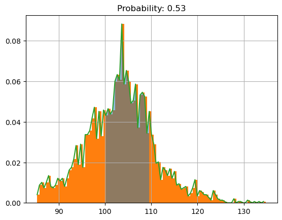
Example: compute the probability of the event 100 < sound level < 110.
The area under heights of the histogram bars and between those bounds will roughly correspond to the empirical probability of this event.
bound_lower = 100
bound_upper = 110
# calculate normalized histogram and store values
h = sound_levels[' BB_20-24000 '].hist(bins=100, density=True)
plt.title("Sound Level Normalized Histogram")
h = plt.hist(sound_levels[' BB_20-24000 '].values, bins=100, density=True)
plt.plot(h[1][:-1], h[0],)
plt.fill_between(h[1][:-1], h[0], where=((h[1][:-1]>bound_lower) & (h[1][:-1]<bound_upper)), alpha=0.5)
p = sum(h[0][(h[1][:-1]>bound_lower) & (h[1][:-1]<bound_upper)])/sum(h[0])
_ = plt.title("Probability: {:.2f}".format(p))
Empirical Probability Widget#
We will use a widget to explore the empirical probability for arbitrary intervals.