The lives of orcas through the SONAR equation

How does the SONAR equation help understand the lives of orcas? Let’s first consider the scenario of Oli trying to communicate with Ola, and examine how different terms in the SONAR equation come into play:

Here, \(SL\) characterizes how loud Oli is calling, \(TL\) describes how much sound energy is “lost” before the sound reaches Ola, and \(RL\) represents how loud the sound is when Ola receives. Depending on what the environment Oli and Ola are in, the content of Oli’s signal (e.g., spectrum), Ola may or may not be able to hear Oli, or hear clearly what Oli is saying.

For example, if they are in a shallow channel, Oli’s sound may bounce around between the sea surface and seafloor (“multipath” propagation) and cause Ola to hear multiple copies of the same sound. It also turns out that Oli’s sound may not reach as far in warmer water compared to in colder water. You will learn more about these in the following sections.

What if we want to predict how far we can detect Oli? It’s pretty straightforward: just replace Ola with a hydrophone:

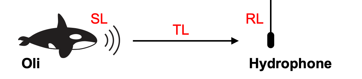
But of course, we need to consider if Ola and the hydrophone receives sound the same way, just like different people may hear the same sound differently.

Now let’s consider the scenario where Ola wants to detect and track down a fish. The picture then changes to the following:

In this case, instead of Oli making a sound, now we have Ola’s echolocation signal bouncing off the fish, characterized by \(\textrm{TS}\). Because the sound now travels both from Ola to the fish, and from the fish to Ola, the amount of sound energy loss doubles, represented by \(\textrm{2TL}\). Similarly, depending on the environment Ola is in and the type and number of fish there are, the exact situation may be more complex then what is depicted here. You will also learn more about these in the following sections.