Rough surface scattering

We will shift now from scattering from discrete objects in the water column such as fish to scattering from the ocean sea surface and seafloor. In both cases, we are measuring sound energy that is redirected by the scatterer. In the case of fish as a scatterer, the refdirected sound is treated as coherent and given the same geometry and if the fish are similar to one another, the redirected sound will appear approximately the same for each fish.

This isn’t the case for the seafloor or the sea surface. As the sea surface changes due to passing waves, the scattered sound can fluctuate significantly. Similarly for the seafloor. Although a large area may have the same statistical description, as the sonar moves over the seafloor, the returned signal will fluctuate.

As a result, instead of treating each returned signal in isolation, the goal of characterizing the scattering is to understand how the statistics of those fluctuations depend on the environment.

Defining and measuring a rough surface

Before we talk about the scattering of sound from the seafloor, we will begin by defining what we mean when we say a rough surface. For the sea surface, while there are occasions when the sea is very calm and the ocean surface is flat, but more often than not, there are waves coming from different directions which creates an undulating surface like the one shown below.

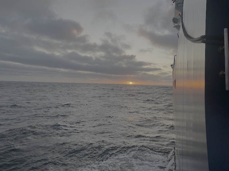
The height of the surface is changing over time and these variations can be treated as random at any point in time or at different locations on the surface. Given this random nature, we use statistics to describe the surface. We can write the height of a random surface as

\[z\left(x,y\right) = \left<z\right> + \delta z\left(x,y\right)\]

where \(\left<z\right>\) is the mean height surface and \(\delta z\) is the displacement of the surface at each point and \(<\delta z> = 0\). We can get a sense of how rough the surface is by looking at the RMS roughness:

\[ h = \sqrt{\left<\delta z\right>^2}. \]

On the right side of the image below is a map of the seafloor height measured using the laser line scanning system shown in the left of the image. This imaging system measures the height of the seafloor at every 1 mm step in the x and y directions. You can clearly see small undulations that might have been produced by currents and circular, pock marks made by feeding fish. For this surface, the RMS roughness is \(h = 0.31\) cm. The sea surface shown above, probably has an rms roughness closer to 10 cm. Rough seas can have RMS roughness on the order of 3-5 m.

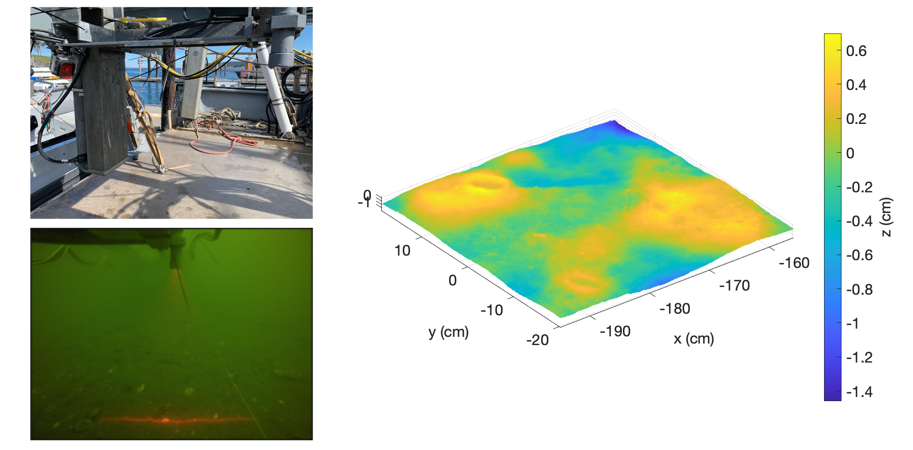
Another way to characterize the roughness of a surface is to look at the roughness power spectrum. While we won’t go into a lot of detail here, the power spectrum is related to the fourier transform of the surface and is a way to see how the fluctuation of the heights on the surface vary as a function of length scale. For example there may be large undulating features on the seafloor that vary horizontal over meters, while there might also be smaller bumps and ridges that change on the order of centimeters. In the example above, the fish pock marks are on the order of 2-10 cm while the larger hill-like features are 20-30 cm long. We will dig into this in greater detail in future versions of this page.

Scattering strength

As we said earlier, sound scattered from a rough surface varies as the rough surface changes in time or if we move to different locations on the surface. As a consequence we are interested in measuring the fluctuations in the scattered field. The total pressure after sound has interacted with the seafloor can be expressed as

\[ p = \left<p\right> + p_s, \]

where \(p_s\) is the scattered pressure and \(<>\) denotes the mean taken using measurements of the recieved pressure from a bunch of different “looks” at the rough surface. This could mean making repeat measurements at the same location on the sea surface as the surface changes due to the passing waves or making measurements at different locations on the seafloor. From this equation, the mean of the scattered pressure is zero. What is of interest in rough surface scattering is not the mean of the scattered pressure, but rather the mean square of the scattered pressure. The mean square scattered pressure can be related to the rough surface properties through

\[<|p_s|^2> = |p_i|^2 A \sigma \frac{1}{r^2},\]

where \(|p_i|^2\) is the mean square of the incident pressure, \(A\) is the area of the scattering patch on the seafloor, \(r_s\) is the distance of the receiver from the patch, and \(\sigma\) is the scattering cross section. This cross section differs from the target scattering cross section in that this cross section is dimensionless since it is now defined for an area. If you wanted to be really specific, you could refer to this as the “scattering cross section per unit area per unit solid angle,” but this is a mouthful and tend to use just “scattering cross section.” The scattering cross section is a function of the incident and scattered grazing angles as was the case in target scattering. Instead of target strength, though, we define the scattering strength as

\[ S = 10\log_{10}\sigma.\]

It’s worth noting that the equation relating the scattered pressure and the scattering cross section is defined in terms of an incident and scattered plane waves. As a result, some care needs to be taken when calculating the scattered field so that the directionality and time dependence of the incident field are taken into account. In the simplest case, the contribution from a small patch of the seafloor can be expressed in terms of the sonar equation as

\[ RL = SL + 2TL + S + 10\log_{10}A,\]

where \(A\) is the area of ensonified patch of the seafloor.

Backscattering from a rough surface

We won’t go into details here, but below is a widget that calculates the backscattering strength for a rough seafloor using a statistical description of the seafloor that yields an RMS roughness of 1 cm. The calculation uses a small roughness perturbation theory and is a good approximation when the ratio of the RMS roughness to the wavelength is small. For the 40 kHz signal used in this example, the wavelength is 3.75 cm and the ratio is \(h/\lambda = 0.27\). The main goal of the widget at this stage is to show how the scattering changes with sediment properties while keeping the rough surface the same.

Show code cell source

Hide code cell source

# Import packages
import numpy as np
import matplotlib.pyplot as plt
import ipywidgets as widgets

# Set inline
%matplotlib inline

Show code cell source

Hide code cell source

def RCoeff(frequency, theta_i_degrees, cw, cp1, rho_ratio, rhow, alphap1):
    """
    Function to compute reflection coefficient.
    """
    # Convert attenuation to loss parameter
    deltap1 = alphap1 * cp1 * np.log(10) / (40 * np.pi * frequency)

    # Convert from degrees to radians
    theta_i = np.deg2rad(theta_i_degrees)

    # Complex sound speed
    cpp = cp1 / (1 + 1j * deltap1)

    # Ratio of sound speeds
    ap = cpp / cw

    # Impedance for water
    zw = rhow * cw / (np.sin(theta_i))

    # Impedance of sediment
    zp = rho_ratio * rhow * cpp / np.sqrt(1 - (ap * np.cos(theta_i))**2)

    # Impedance ratio
    zwp = zp / zw

    # Reflection coefficient
    R1 = (zwp - 1) / (zwp + 1)

    return R1

Show code cell source

Hide code cell source

def perturb_roughness_scattering(frequency, theta_i_degrees, theta_s_degrees, phi_s, cw, cp1, rho_ratio, rhow, alphap1, w2, gamma2, L2):
    """
    Function to compute the roughness scattering cross section using perturbation theory"
    """
    # Convert attenuation to loss parameter
    deltap1 = alphap1 * cp1 * np.log(10) / (40 * np.pi * frequency)

    # Convert from degrees to radians
    theta_i = np.deg2rad(theta_i_degrees)
    theta_s = np.deg2rad(theta_s_degrees)

    # Ratio of sound speeds
    ap = cp1 / (cw * (1 + 1j * deltap1))

    # Wavenumber
    kw = 2 * np.pi * frequency / cw

    ## Reflection coefficients for theta_i and theta_s
    Vww_i = RCoeff(frequency, theta_i_degrees, cw, cp1, rho_ratio, rhow, alphap1)
    Vww_s = RCoeff(frequency, theta_s_degrees, cw, cp1, rho_ratio, rhow, alphap1)

    # sin(theta_{pi}) and sin(theta_{ps})
    stpi = np.sqrt(1 - (ap * np.cos(theta_i))**2)
    stps = np.sqrt(1 - (ap * np.cos(theta_s))**2)

    # Coefficients
    B = stpi * stps /(np.square(ap) * rho_ratio)

    G = (1 - 1 / rho_ratio) * (np.cos(theta_i) * np.cos(theta_s) * np.cos(phi_s) - B) - 1 + (1 / (np.square(ap) * rho_ratio))

    Aww = (1 + Vww_i) * (1 + Vww_s) * G / 2

    # incident wavenumber
    ki_x = kw * np.cos(theta_i)
    ki_y = 0;
    
    # scattered wavenumber
    ks_x = kw * np.cos(theta_s) * np.cos(phi_s)
    ks_y = kw * np.cos(theta_s) * np.sin(phi_s)

    # Bragg wavenumber
    dK = np.sqrt((ks_x - ki_x)**2 + (ks_y - ki_y)**2)

    # Spectral Level
    W_dK = w2 / ((dK**2 + (2 * np.pi / L2)**2)**(gamma2 / 2))

    # Backscattering cross section
    sigma = (kw**4) * (np.abs(Aww)**2) * W_dK
    
    return sigma

Show code cell source

Hide code cell source

def plot_scattering_strength(cp1, rhop1, alphap1):
    """
    # Function to plot magnitude and phase of the reflection coefficient and show critical / intromission angles.
    """

    # Frequency
    frequency = 40

    # Water sound speed (m/s)
    cw = 1500

    # Water density (kg/m^3)
    rhow = 1000

    # Density ratio
    rho_ratio = rhop1 * 1000 / rhow

    # Grazing angles for reflection coefficient
    theta = np.arange(0.25, 60, 0.25)

    # Set phi_s = pi for backscatter
    phi_s = np.pi

    # Spectral Strength (m^(4-\gamma2))
    w2 = 0.0021

    # Spectral exponent
    gamma2 = 4.23

    # Cutoff Length (m)
    L2 = 1

    # 
    sigma = perturb_roughness_scattering(frequency * 1000, theta, theta, phi_s, cw, cp1, rho_ratio, rhow, alphap1, w2, gamma2, L2)

    # Close any existing plots
    plt.close('all')

    # Plotting
    plt.figure(1)
    plt.plot(theta, 10 * np.log10(sigma), linewidth=2)
    plt.xlabel('Grazing Angle (degrees)')
    plt.ylabel('Scattering Strength (dB)')
    plt.grid(True)
    
    plt.show



# Create interactive widgets
layout = widgets.Layout(width="500px", height="30px")
widgets.interact(
    plot_scattering_strength,
    cp1=widgets.FloatSlider(
        min=1300,
        max=1750,
        step=1,
        value=1720,
        description="Sediment Speed (m/s)", 
        style={"description_width": "initial"}, 
        layout=layout,
    ),
    rhop1=widgets.FloatSlider(
        min=1.2,
        max=2.5,
        step=0.1,
        value=2.1, 
        description="Sediment Density (g/cm^3)", 
        style={"description_width": "initial"}, 
        layout=layout,
    ),
    alphap1=widgets.FloatSlider(
        min=20,
        max=650,
        step=10,
        value=20, 
        description="Attenuation (dB/m)", 
        style={"description_width": "initial"}, 
        layout=layout,
    ),
)

<function __main__.plot_scattering_strength(cp1, rhop1, alphap1)>

A couple of things are worth mentioning here:

1. The scattering strength decreases with decreasing grazing angle.

2. The reflection coefficient plays an important role. When there is a critical angle, \(c_s > c_w\), where \(c_w = 1500\) m/s in this case, there is a pronounced “bump” in the scattering strength at the critical angle. As the sound speed is decreased below the water sound speed, the scattering strength drops appreciably.

3. While we don’t see it in this calculation, as the frequency gets lower, the scattering strength decreases. Another way of thinking about this is that as the wavelength of the sound increases, the surface appears smooth to the incoming wave.