Discrete scatterers#
What are discrete scatterers and why they matter#
We call something a discrete scatterer when we consider its scattering response on its own, without other scattering sources nearby. Discrete scatterers are extremely useful, because not only can we model individual things in the ocean—a bubble, oil droplet, sand, fish, krill, whale, or even a submarine—as discrete scatterers, we can also model the combined scattering from a group of these things as a collection of discrete scatterers. This allows us to build up models for more complex scenarios, like a patch of seafloor or sea surface, a cloud of bubbles or a school of fish.
When working with discrete scatterers, we often approximate them as point scatterers that can be isolated from the rest of the ocean acoustics “system.” This way, we can think of a scatterer as a new sound source that radiates sound after it is excited by the incident waves, and can immdiately apply the many concepts we have learned in the Acoustic sources section here, such directionality.
Modeling real-world scatterers#
When trying to interpret echograms, we usually rely on a set of expectations based on the environment and physics to help us understand what we are seeing. Specifically, we consider:
The environmental context that influences the types of objects that are likely to occur, such as bathymetry, geographical region, season, etc.
How different types of objects scatter sound (i.e. acoustic scattering models)
For example, near an estuary, we may expect to see strong scattering from suspended sediments that have been stirred up by the water flows; near a fishing ground, we may expect to see strong scattering from fish schools.
Archetypes#
There are so many different types of objects and animals in the ocean. How do we model them? It turns out that the rules of physics have helped us construct a few archetypes that are really useful in thinking about how something scatterers sound. These are:
Scatterers with compressible air cavities, such as bubbles and fish with swimbladder.
“Fluid-like” scatterers that have material properties similar to the surrounding water, such as squid, jellyfish, krill, oil droplets, etc.
Scatterers containing “elastic” materials that supports both compressional and shear waves, such as shells and dense mineral particles.
On top of these, we consider the sizes and shapes of scatterers, and importantly, make approximation when we can to simplify the problem. For example, fish swimbladders are seldom spherical, but at low frequencies, approximating it as a bubble gives pretty good results; krill or shrimps have elongated bodies and many thin legs, but approximating them as fluid-like spheroids also gives pretty good results.
We will explore these properties below.
Size dependency#
The mighty \(ka\)#
When we talk about the size of a scatterer, we are really taking about the relative size of a scatterer with respect to the acoustic wavelength. We often use a dimensionless number, \(ka\), to quantify the relative size. Here,
\(k=2\pi/\lambda\) is the acoustic wavenumber, which represents the phase within a wavelength, and
\(a\) is the characteristic dimension of a scatterer, such as the radius of a sphere or the length of a cylinder.
\(ka\) is dimensionless, because both \(\lambda\) and \(a\) are length measures with units of \(\textrm{m}\). This allows us to easily compare the echo reponse of a large scatterer at low frquency and a small scatterer at high frequency — not based on the absolute size of the scatterer, but based on the ratio between wavelength and scatterer size.
This is such an important concept that we encourage you to try the widget below again, to remind yourself about what phase angle is and its relationship with the wavenumber \(k\).
<function __main__.plot_wave_and_circle(x_val)>
scattering regimes#
The scattering response of a given scatterer can be generally described based on the scattering regimes across frequency:
In the Rayleigh regime, the acoustic wavelength is very large compared to the scatterer (\(ka\ll1\)), and the scattering is dominated by diffraction. Here, the exact shape of the scatterer is often not as critical in determining the scattering response, and the scattering cross section scales with frequency with a steep slope proportional to \((ka)^4\).
In the geometric regime, the acoustic wavelength is small compared to the scatterer (\(ka\gg1\)), and the scattering is dominated by reflection. Here, the scattering cross section typically oscillates around a high-frequency limit, with deep spectral nulls due to interference from surface waves or other reflections within the target depending on its material properties.
The figures below show the target strength of a solid tungsten carbide sphere plotted in both linear and log scale along the x-axis. Such spheres are commonly used for calibrating high-frequency sonar systems, since its scattering response can be accurately modeled.
On log-scale plot (left), we can easily see the \((ka)^4\) dependency of the Rayleigh regime.
On the linear-scale plot (right), we can find frequency sections where the TS does not vary rapidly, which are useful for calibration.
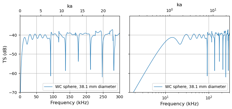
Exercise
Look at the linear-scale plot, can you guess why it is usually not recommended to calibrate a system with transmit frequencies near one of the TS spectral nulls?
Influence of material properties#
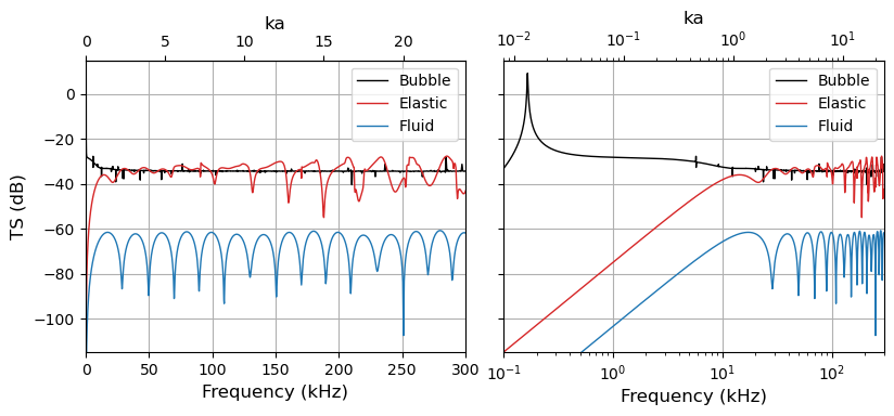
Scattering phenomena can vary strongly depending on the material composition of scatterers. The figure below shows the TS of spheres of the same size but different material properties:
Bubbles, or any scatterers that include a compressible air cavity, can resonate in the \(ka\ll1\) region, producing scattering signals much stronger than similarly sized objects without air.
“Fluid-like” scatterers are made of materials very similar to the surrounding water medium, which allows sound to easily transmit and reflect through, causing regular interference patterns seen on the TS spectrum.
“Elastic” scatterers contain dense materials, such as bones, steel or tungsten carbide we saw above, which support complex surface waves that result in complex patterns on the TS spectrum.
Most scatterers contain more than one type of materials, and there the question is whether some mechanisms dominate over the others, and which they are.
Exercise
To get an intuitive feel of how the echoes change depending on the scatterer, use the widget below to answer the following questions:
How does the resonance frequency of the gas bubble change as its radius increases or decreases?
What is the approximate size of a bubble that gives a resonance around 10 Hz?
How does the TS spectral pattern of the fluid sphere change as its radius increases or decreases?
Orientation dependency#
In the above we only discussed the scattering of spheres. However, most scatterers in nature are not spherical. What does a non-spherical shape do to the scattering response?
As you may have expected intuitively, echoes from non-spherical scatterers would very depending on the incident angle. This is especially true when \(ka\) is high, meaning that the wavelength is small compared to the size of the scatterer.
Exercise
To get an idea of how scattering directionality looks like, try the widget below to see how TS changes as a function of frequency and incident angle.
How does directionality change (stronger or weaker) with increasing frequency?
How does the TS spectrum change with increasing angles?
Exercise
The size and the aspect ratio of the fluid prolate spheroid also strongly affect its directionality. Use the widget below to answer the following questions:
How does the directionality at the same frequency change as the spheroid becomes bigger, or when its aspect ratio becomes larger?
Thinking back on what you learned about phase difference and interference between waves, can you guess why?
Inferring scatterer identity#
Seeing how the TS spectrum can change with size, material properties, shape, and incident angle for simple scatterers, such as spheres and spheroid, we can use these features to infer the identity of scatteres, or the dominant scattering mechanisms within a scatterer.
Acoustic color#
For example, the variation of TS spectrum across angle has been referred to as “acoustic color” and used to find unexploded ordnance (UXO) underwater. Below you can see the comparison of experimentally measured acoustic color and two model predictions of a small aluminum replica of an UXO (adapted from Fig. 5 of Kargl et al. 2014).
Multi-frequency narrowband observation#
In scenraios where the instruments cannot capture scattering responses over a wide frequency range (broadband), we may opt for comparing the scattering response across multiple narrower frequency bands (narrowband). In fact, many fisheries echosounders use narrowband signals spaced out across a large frequency range to try to observe animals from krill to whales that vary dramaticaly in size and anatomical compositions.
Exercise
In the widget below, you are seeing the same “slice” of the ocean through three different narrowband frequencies. Let’s try to infer the scatterer identity using the series of questions below:
The swimbladdered fish in this environment are typically much larger than krill (a small zooplankton with fluid body). How do you think the scattering response of fish and krill compare at lower frequency?
Based on your answer above, which part of the echogram do you think is dominated by fish?
Observe the change of echo strength with increasing frequency. Based on what you know about the echo response of fluid-like scatterers, which part of the echogram do you think is dominated by krill?
For the fish part of the echogram you have identified, how does the echo response change with frequency, and why? (Hint: fish swimbladder is usually elongated and therefore are directional, especially at higher frequencies.)
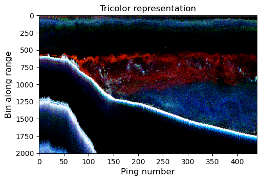
Based on intuition from the above, some fisheries scientists create a “tricolor” representation of the echogram by mapping the echo strengths at three frequencies into the RGB colors, which conveniently summarizes the spectral information.
Exercise
Can you use the tricolor representation to quickly tell which part of the echogram is likely dominated by fish and zooplankton, respectively?